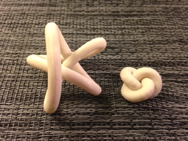
Two more trefoil conformations – as a petal knot (all crossings line up along one center stem) and a tight knot (with the smallest amount of rope length possible given its diameter):
STL file for petal: http://www.geekhaus.com/makerhome/day152_trefoil_petal_40_25_3.stl
STL file for tight: http://www.geekhaus.com/makerhome/day152_trefoil_minimumrope_25.stl
Thingiverse link: http://www.thingiverse.com/thing:234107
Settings: MakerWare .3mm/low in 20-25 minutes for the petal knot and even less for the tight knot, with the minimum-support custom slicing profile for knots described on Day 110.
Technical notes, math flavor: The beautiful petal knot conformation is from the paper Bounds on Übercrossing and Petal Numbers for Knots by Colin Adams at Williams College and his amazing team of student researchers. In this work Adams, et al made the startling decision to study “petal” projections of knots where the crossings occur all on top of each other in one place! This is a wild and crazy idea compared to the usual notion that we should look at knot projections where crossings happen nicely and one at a time. But this crazy idea bore some amazing fruit: they proved that every knot admits a petal projection, and went on to discover deep connections between the übercrossing number of knots and other traditional invariants such as crossing and unknotting numbers. I know I’m not supposed to have favorites, but of the eight trefoil knots I am printing in this collection, this is by far my favorite. It’s beautiful and surprising each time you turn the knot over and the perspective shifts from one-crossing-at-a-time to all-crossings-lined-up-at-once. Wonderful! See the OpenSCAD code below if you want a (piecewise) parametrization of this knot.
Minimum-length rope knot conformations of the tiny trefoil aren’t the most impressive, but for higher-crossing knots they are fascinating, and what started my journey with 3D printing last year. Jason Cantarella at the University of Georgia and Eric Rawdon at the University of St. Thomas, together with some students, have been investigating “tight” knots since their paper Knot Tightening by Constrained Gradient Descent in which they used their ridgerunner algorithm to find minimal conformations of a large number of knots. The data they made available with this paper was what helped me model my first 3D-printable knot models (for example, see Day 9, Day 11, Day 66, and Day 67).
Technical notes, OpenSCAD flavor: By the time of this posting, kitwallace and the GitHub OpenSCAD community had improved this code significantly; see kitwallace’s excellent post at his blog The Wallace Line. However the new code requires the new 2014.01.04 snapshot of OpenSCAD, which does not want to work on my machine at the moment. Therefore I will post the old, slow code. It works but it ain’t fast. In fact, it ain’t pretty either, since getting Adams’ petal knot parametrization to work in OpenSCAD required creating a very clunky piecewise function, as you will see in the code below. And it just gets worse for the tight knot; I have a very inefficient piece of code that takes 50 coordinates from Cantarella’s data and connects the dots with hulled pairs of spheres. I am sure a nice loop would have made quicker work of the problem, but at the time my clunky mess of code was easier to write. I’ve put that code under the fold so you have to click through to see my code of shame.
// mathgrrl parametric knots
// tubify module based on tube module from kitwallace
// choose the knot you want and comment out the rest
// trefoil as petal knot
// http://arxiv.org/pdf/1311.0526v1.pdf
// based on mma algorithm from Adams, need to do z-coord in cases
// scaled to 40mm before tubifying
tempstep = .005; //.005/1 is 2/360
function g(t,a,b,u,v) =
[ 3.5*5*cos(180*t)*sin(5*180*t),
3.5*5*sin(180*t)*sin(5*180*t),
8*u*(cos(180*(((5*t-a+1)%5)-1)/2))*(cos(180*(((5*t-a+1)%5)-1)/2))
+ 8*v*(cos(180*(((5*t-b+1)%5)-1)/2))*(cos(180*(((5*t-b+1)%5)-1)/2))
];
translate([0,0,-24])
union(){
color(“red”)
for (t=[1: tempstep: 1.2-tempstep]) { //replacement for 0 to .2
hull() {
translate(g(t,5,1,4,1)) sphere(2.5);
translate(g(t+tempstep,5,1,4,1)) sphere(2.5);
}
}
color(“orange”)
for (t=[.2: tempstep: .4]) { //also why here?
hull() {
translate(g(t,1,2,1,3)) sphere(2.5);
translate(g(t+tempstep,1,2,1,3)) sphere(2.5);
}
}
color(“yellow”)
for (t=[.4: tempstep: .6]) {
hull() {
translate(g(t,2,3,3,5)) sphere(2.5);
translate(g(t+tempstep,2,3,3,5)) sphere(2.5);
}
}
color(“green”)
for (t=[.6: tempstep: .8]) {
hull() {
translate(g(t,3,4,5,2)) sphere(2.5);
translate(g(t+tempstep,3,4,5,2)) sphere(2.5);
}
}
color(“blue”)
for (t=[.8: tempstep: 1]) {
hull() {
translate(g(t,4,5,2,4)) sphere(2.5);
translate(g(t+tempstep,4,5,2,4)) sphere(2.5);
}
}
}
——————
As an Amazon Associate we earn from qualifying purchases, so if you’ve got something you need to pick up anyway, going to Amazon through this link will help us keep Hacktastic running. Thanks! :)


you have lots of perseverance!
can you print the Lorenz attractor come from the chaos theory.
i think it is very special but also hard.