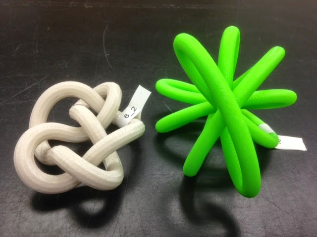
Today is my favorite from the 3D-Printed Conformations of Knots through 7 Crossings series that my Math 297 students developed last semester in the JMU 3-SPACE classroom. It’s a petal knot conformation of 6_2, which means that there is an angle from which all of the crossings line up on top of one another to form a single daisy-like crossing. Colin Adams of Williams College, together with an army of amazing students, proved recently that every knot has a petal conformation. They also came up with explicit constructions for some of those conformations, one of which we used to print today’s model:
Thingiverse link: http://www.thingiverse.com/make:80268
Settings: Printed on a Replicator 2 with our usual custom knot slicing profile.
Technical notes, Mathematica flavor: Today’s petal knot was designed and printed by JMU Student Jonathan Gerhard, using the method from Day 152 and data sent to us by Adams’ student Daniel Vitek. Here’s Jonathan’s walkthough of what he did:
The data for the petal knot conformation of 6_2 came in the form of 500 points in space determined by the following Mathematica code:
Bumps[t_, n_] := If[Abs[Mod[t, n, -n/2]] > 1, 0, Cos[π*Mod[t, n, -n/2]/2]^2];

BumpSum[p_, t_] := Sum[p[[i]]*Bumps[t + 1 - i, Length[p]], {i, 1, Length[p]}];

PetalPlot[p_] := ParametricPlot3D[{
 Sin[π*t]*Cos[π*t/Length[p]],
 Sin[π*t]*Sin[π*t/Length[p]],
 BumpSum[p, t]},
 {t, 0, Length[p]}];

p = {1, 3, 5, 2, 8, 4, 7, 9, 6};

points = N[{Sin[π*t]*Cos[π*t/Length[p]], Sin[π*t]*Sin[π*t/Length[p]],
     BumpSum[p, t]} /. ({t -> #} & /@ (Range[0, 500]/500*Length[p]))];

ListPointPlot3D[points]

To get a smooth representation we could just use Tube in Mathematica, as follows:
Graphics3D[Tube[points, .075]]

This looked good, however, it was very tall. So I modified it by changing the BumpSum[p, t]} in PetalPlot[p_] to 0.26BumpSum[p, t]}to make the height smaller.
Mathematica models can sometimes export badly, so instead of using the Tube model above I used the OpenSCAD technique we’ve been using for our data-defined knots (see for example Day 272). To do this, I first had to open the 500 Mathematica datapoints in TextEdit and run a “Find and Replace” to change all “{“s to “[“ and all “}” to “],”s. Then I input the reformatted data points into the following OpenScad code (not all of the points are included here because there are so many!):
Paths = [[
[0., 0., 0.26],[0.05651741885454146, 0.00035511408887296787, 0.26041559697166655],[0.11284747420775955, 0.0014181578334111625, 0.2616610592647978],[0.16880345185324083, 0.0031822470046126636, 0.2637324052612605],[0.22419993383963085, 0.005635945627807872, 0.2666230130754899],[0.27885344076990115, 0.008763322416738774, 0.27032364172399476],
%...lots of data points
[-0.27885344076990115, 0.008763322416738774, 0.28580910430998696],[-0.22419993383963085, 0.005635945627807872, 0.27655753268872485],[-0.16880345185324083, 0.0031822470046126636, 0.26933101315315133],[-0.11284747420775955, 0.0014181578334111625, 0.2641526481619946],[-0.05651741885454146, 0.00035511408887296787, 0.26103899242916623],[0., 0., 0.26],[0.05651741885454146, 0.00035511408887296787, 0.26041559697166655],
]];
// Sides of the tube
Sides = 30;
// Radius of tube
Radius = .1;
//Scale of knot
Scale= 3;

Colors = [[1,0,0],[0,1,0],[0,0,1],[1,1,0],[1,0,1],[0,1,1]];
module disc_p2p(p1, p2, r) {
  assign(p = p2 - p1)
  translate(p1 + p/2)
    rotate([0, 0, atan2(p[1], p[0])])
    rotate([0, atan2(sqrt(pow(p[0], 2)+pow(p[1], 2)),p[2]), 0])
    render() cylinder(h = 0.1, r1 = r, r2 = 0);
};

module knot_path(path,r) {
  for (t = [0: 1: len(path)-1 ])
    assign (p0 = path[t],
      p1 = path[(t + 1) % len(path)],
      p2 = path[(t + 2) % len(path)] )
    hull() {
      disc_p2p (p0,p1,r);
      disc_p2p (p1,p2,r);
    }
};

module knot(paths,r)
  for (i = [0:1:len(paths)-1])
    color(Colors[i])
     knot_path(paths[i],r);

$fn=Sides;
scale(Scale)
knot(Paths,Radius);
Compile and render this by hitting “F6”. Once it finishes (which will take forever), go to the OpenSCAD Design menu and choose “Export as STL”. And you’re done!


Leave a Reply